Level: Beginner
This is my first part, on an initiative to start introducing my viewers to few of the areas where I have had some experience and learning. Lets start with the understanding, definition and history behind to understand it better.
What is a spreadsheet?
A spreadsheet is basically a computer application, used for analysis of data represented in tabular form. Spreadsheets were initially developed as computerized simulations of paper accounting worksheets.
The program operates on data represented as cells of an array, organized in rows and columns. Modern spreadsheet software can have multiple interacting sheets, and can display data either as text and numerals, or in graphical form.
Microsoft Excel is one such modern spreadsheet product from Microsoft, which is widely used by almost all professionals and home users alike. We will be talking about MS Excel and all references to spreadsheet should be read as, in purview of MS Excel only. An Excel file consists of multiple worksheets (usually called sheets) that make up one workbook, with each file being one workbook.
History (Quoted from Wiki)
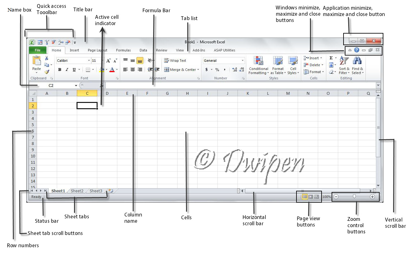
Now lets identify parts of the Excel screen, which has been labelled as below for easy understanding.

Introduction to the Ribbon tabs
The Ribbon is grouped into different related tabs. Lets have a small overview of the tabs.
Home: This is the default tab, whenever you open Excel. This tab contains the basic Clipboard commands, font formatting and alignment commands, commands to insert and delete rows or columns lastly worksheet editing commands.
Insert: This tab will help you insert something in a worksheet -a table, diagram, chart, symbol, and so on.
Page Layout: This tab contains basic tools and commands to change the appearance of your worksheet, including printing.
Formulas: This tab is used to insert a formula, use or name range, access formula tools and control performs calculations.
Data: Data-related commands and manipulation tools are on this tab.
Review: This tab has tools to review your work, check spelling, translate words, add comments, or protect sheets.
View: This tab contains commands that will help you control various views of how a sheet is viewed.
Developer: This isn’t visible by default, and can be enabled from Excel options. It contains commands that are useful for programmers.
Add-Ins: This is visible only if you’ve loaded a workbook or installed an add-in.
Create the first worksheet.
Open Excel and create a new, blank workbook, by pressing Ctrl+N.
Inorder to work on Excel, we need to have some data, so let us take an example of a retail shop where the sales volume is available for a year. It will hence will have two columns of information; Column A will contain the month names, and column B will store the sales volumes.
Lets begin each step as below
1. Move the mouse to cell A1 by using the direction keys. The Name box will display the cell’s
address as A1.
2. Enter label of the table as Month into cell A1. Just type the text "Month" and then press Enter.
3. Now move the cell pointer to B1, type "Sales volume" and press Enter.
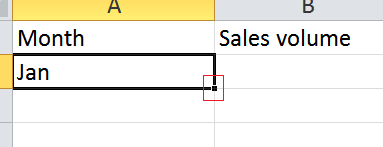
1. Move the mouse to A2 and type Jan (abbreviation for January).
2. When you select the cell A2 is selected, observer that the active cell is displayed with a heavy outline.
Check the bottom-right corner of the cell outline, you’ll see a small square known as the fill handle. Now move the mouse pointer over the fill handle, click and without releasing it, drag down until you’ve highlighted cells from A2 down to A13.
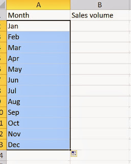
3. Release the mouse button, and Excel will automatically fill in the month names.
Your worksheet should resemble the one shown below.
Entering the sales data
Lets fill out the sales volume in the next column. Lets assume that January’s sales volume is 2,000, and that it will increase by 3.5 percent in each of the subsequent months. This is how we will take it ahead.
1. Move the mouse to B2 and type 2000 , the sales volume for January.
2. To calculate the projected sales, we need to enter a formula for February. Move to cell B3 and enter
the following: =B2*103.5%. When you press Enter, the cell will display 2070. The formula
returns the contents of cell B2, multiplied by 103.5%. In other words, February sales are projected
to be 3.5% greater than January sales.
3. The projected sales for subsequent months will use a similar formula. But rather than retype
the formula for each cell in column B, once again take advantage of the AutoFill feature (done for Month column). Ensure that cell B3 is selected. Click the cell’s fill handle, drag down to cell B13, and release the
mouse button.
Your worksheet should now be looking like the one below. To check the formulas, you can try changing the projected sales value for the initial month, January (in cell B2). You’ll find that the formulas recalculate and return different values. But these formulas all depend on the initial value in cell B2.

Happy learning, shall continue with more in second part. Please feel free to comment or ask questions.
This is my first part, on an initiative to start introducing my viewers to few of the areas where I have had some experience and learning. Lets start with the understanding, definition and history behind to understand it better.
What is a spreadsheet?
A spreadsheet is basically a computer application, used for analysis of data represented in tabular form. Spreadsheets were initially developed as computerized simulations of paper accounting worksheets.
The program operates on data represented as cells of an array, organized in rows and columns. Modern spreadsheet software can have multiple interacting sheets, and can display data either as text and numerals, or in graphical form.
Microsoft Excel is one such modern spreadsheet product from Microsoft, which is widely used by almost all professionals and home users alike. We will be talking about MS Excel and all references to spreadsheet should be read as, in purview of MS Excel only. An Excel file consists of multiple worksheets (usually called sheets) that make up one workbook, with each file being one workbook.
History (Quoted from Wiki)
The word "spreadsheet" came from "spread" in its sense of a newspaper or magazine item (text and/or graphics) that covers two facing pages, extending across the center fold and treating the two pages as one large one. The compound word "spread-sheet" came to mean the format used to present book-keeping ledgers—with columns for categories of expenditures across the top, invoices listed down the left margin, and the amount of each payment in the cell where its row and column intersect—which were, traditionally, a "spread" across facing pages of a bound ledger (book for keeping accounting records) or on oversized sheets of paper (termed "analysis paper") ruled into rows and columns in that format and approximately twice as wide as ordinary paper.
Now lets identify parts of the Excel screen, which has been labelled as below for easy understanding.
Introduction to the Ribbon tabs
The Ribbon is grouped into different related tabs. Lets have a small overview of the tabs.
Home: This is the default tab, whenever you open Excel. This tab contains the basic Clipboard commands, font formatting and alignment commands, commands to insert and delete rows or columns lastly worksheet editing commands.
Insert: This tab will help you insert something in a worksheet -a table, diagram, chart, symbol, and so on.
Page Layout: This tab contains basic tools and commands to change the appearance of your worksheet, including printing.
Formulas: This tab is used to insert a formula, use or name range, access formula tools and control performs calculations.
Data: Data-related commands and manipulation tools are on this tab.
Review: This tab has tools to review your work, check spelling, translate words, add comments, or protect sheets.
View: This tab contains commands that will help you control various views of how a sheet is viewed.
Developer: This isn’t visible by default, and can be enabled from Excel options. It contains commands that are useful for programmers.
Add-Ins: This is visible only if you’ve loaded a workbook or installed an add-in.
Create the first worksheet.
Open Excel and create a new, blank workbook, by pressing Ctrl+N.
Inorder to work on Excel, we need to have some data, so let us take an example of a retail shop where the sales volume is available for a year. It will hence will have two columns of information; Column A will contain the month names, and column B will store the sales volumes.
Lets begin each step as below
1. Move the mouse to cell A1 by using the direction keys. The Name box will display the cell’s
address as A1.
2. Enter label of the table as Month into cell A1. Just type the text "Month" and then press Enter.
3. Now move the cell pointer to B1, type "Sales volume" and press Enter.
Tip: Autofill function
As we know, we will be filling the Column A with the months Jan-Dec, I thought it is a good time to chip in a tip to fill it up quickly, instead of manually doing it.1. Move the mouse to A2 and type Jan (abbreviation for January).
2. When you select the cell A2 is selected, observer that the active cell is displayed with a heavy outline.
Check the bottom-right corner of the cell outline, you’ll see a small square known as the fill handle. Now move the mouse pointer over the fill handle, click and without releasing it, drag down until you’ve highlighted cells from A2 down to A13.
3. Release the mouse button, and Excel will automatically fill in the month names.
Your worksheet should resemble the one shown below.


Lets fill out the sales volume in the next column. Lets assume that January’s sales volume is 2,000, and that it will increase by 3.5 percent in each of the subsequent months. This is how we will take it ahead.
1. Move the mouse to B2 and type 2000 , the sales volume for January.
2. To calculate the projected sales, we need to enter a formula for February. Move to cell B3 and enter
the following: =B2*103.5%. When you press Enter, the cell will display 2070. The formula
returns the contents of cell B2, multiplied by 103.5%. In other words, February sales are projected
to be 3.5% greater than January sales.
3. The projected sales for subsequent months will use a similar formula. But rather than retype
the formula for each cell in column B, once again take advantage of the AutoFill feature (done for Month column). Ensure that cell B3 is selected. Click the cell’s fill handle, drag down to cell B13, and release the
mouse button.
Your worksheet should now be looking like the one below. To check the formulas, you can try changing the projected sales value for the initial month, January (in cell B2). You’ll find that the formulas recalculate and return different values. But these formulas all depend on the initial value in cell B2.

Happy learning, shall continue with more in second part. Please feel free to comment or ask questions.